Capstone - Using a RNN Model with Keras for Text Classification
I was curious to see how a Recurrent Neural Network model would perform on the text data from my Classifying Political News Media Text Capstone project, as I know that they are known to work very well with text classification. I used this LSTM model on Kaggle as a template. After preprocessing the text, it is converted to a series of integers with sequence, which is somewhat like how a Hashing Vectorizer works. It is then converted into a NumPy array matrix with padding to ensure it has the right shape for the RNN.
import pandas as pd
import numpy as np
import matplotlib.pyplot as plt
from sklearn.model_selection import train_test_split
from keras.models import Model, Sequential
from keras.layers import LSTM, Activation, Dense, Dropout, Input, Embedding, Conv1D, GlobalMaxPooling1D
from keras.optimizers import RMSprop
from keras.preprocessing.text import Tokenizer
from keras.preprocessing import sequence
from keras.utils import to_categorical
from keras.callbacks import EarlyStopping
from nltk.stem import WordNetLemmatizer
from nltk.tokenize import RegexpTokenizer
from sklearn.feature_extraction.text import ENGLISH_STOP_WORDS
%matplotlib inline
Using TensorFlow backend.
# Load the data
text = pd.read_csv('./data/text2.csv').drop('Unnamed: 0', axis=1)
# Set text features and target
X = text['combined']
y = text['yes_right']
# Train test split
X_train, X_test, y_train, y_test = train_test_split(X, y, random_state=24, stratify=y)
# Preprocess data to remove pre-identified stop grams and stop words
lemmatizer = WordNetLemmatizer()

stop_grams = ['national review','National Review','Fox News','Content Uploads',
                  'content uploads','fox news', 'Associated Press','associated press',
                  'Fox amp Friends','Rachel Maddow','Morning Joe','morning joe',
                  'Breitbart News', 'fast facts', 'Fast Facts','Fox &', 'Fox & Friends',
                  'Ali Velshi','Stephanie Ruhle','Raw video', '& Friends', 'Ari Melber',
                  'amp Friends', 'Content uploads', 'Geraldo Rivera']

def my_preprocessor(doc, stop_grams):
    for ngram in stop_grams:
        doc = doc.replace(ngram,'')
    return lemmatizer.lemmatize(doc.lower())
X_train = [my_preprocessor(n, stop_grams=stop_grams) for n in X_train]
X_test = [my_preprocessor(n, stop_grams=stop_grams) for n in X_test]
# Tokenize, convert to sequence of integers, and then to matrix
max_words = 2000
max_len = 200
tok = Tokenizer(num_words=max_words)
tok.fit_on_texts(X_train)
sequences = tok.texts_to_sequences(X_train)
sequences_matrix = sequence.pad_sequences(sequences,maxlen=max_len)
# This is what our words look like as a sequence and as the matrix
print(sequences[0], '\n')
print(sequences_matrix[1])
[1, 84, 10, 1, 814, 1311, 3, 1151, 371, 748, 1189, 167, 959, 2, 54, 280, 3, 26, 103, 1311]

[   0    0    0    0    0    0    0    0    0    0    0    0    0    0    0
    0    0    0    0    0    0    0    0    0    0    0    0    0    0    0
    0    0    0    0    0    0    0    0    0    0    0    0    0    0    0
    0    0    0    0    0    0    0    0    0    0    0    0    0    0    0
    0    0    0    0    0    0    0    0    0    0    0    0    0    0    0
    0    0    0    0    0    0    0    0    0    0    0    0    0    0    0
    0    0    0    0    0    0    0    0    0    0    0    0    0    0    0
    0    0    0    0    0    0    0    0    0    0    0    0    0    0    0
    0    0    0    0    0    0    0    0    0    0    0    0    0    0    0
    0    0    0    0    0    0    0    0    0    0    0    0    0    0    0
    0    0    0    0    0    0    0    0    0    0    0    0    0    0    0
    0    0    0    0    0    0    0    0    0    0    0    0    0    0    0
    0 1815  362   10 1237   22  271    5 1083    1  150 1083    6 1614   32
   27    1  711 1322  742]
# Make sure it is a numpy array
type(sequence), type(sequences_matrix)
(module, numpy.ndarray)
# Build RNN
# I like using function for these steps; I had not encountered that before
def RNN():
    inputs = Input(name='inputs',shape=[max_len])
    layer = Embedding(max_words,50,input_length=max_len)(inputs)
    layer = LSTM(64)(layer)
    layer = Dense(256,name='FC1')(layer)
    layer = Activation('relu')(layer)
    layer = Dropout(0.5)(layer)
    layer = Dense(1,name='out_layer')(layer)
    layer = Activation('sigmoid')(layer)
    model = Model(inputs=inputs,outputs=layer)
    return model
# Compile model
model = RNN()
model.summary()
model.compile(loss='binary_crossentropy', optimizer='adam', metrics=['accuracy'])
_________________________________________________________________
Layer (type)                 Output Shape              Param #
=================================================================
inputs (InputLayer)          (None, 200)               0
_________________________________________________________________
embedding_1 (Embedding)      (None, 200, 50)           100000
_________________________________________________________________
lstm_1 (LSTM)                (None, 64)                29440
_________________________________________________________________
FC1 (Dense)                  (None, 256)               16640
_________________________________________________________________
activation_1 (Activation)    (None, 256)               0
_________________________________________________________________
dropout_1 (Dropout)          (None, 256)               0
_________________________________________________________________
out_layer (Dense)            (None, 1)                 257
_________________________________________________________________
activation_2 (Activation)    (None, 1)                 0
=================================================================
Total params: 146,337
Trainable params: 146,337
Non-trainable params: 0
_________________________________________________________________
history = model.fit(sequences_matrix, y_train,batch_size=128, epochs=10,
          validation_split=0.2,callbacks=[EarlyStopping(monitor='val_loss',min_delta=0.0001)])
Train on 22112 samples, validate on 5528 samples
Epoch 1/10
22112/22112 [==============================] - 85s 4ms/step - loss: 0.5953 - acc: 0.6692 - val_loss: 0.5288 - val_acc: 0.7315
Epoch 2/10
22112/22112 [==============================] - 87s 4ms/step - loss: 0.4811 - acc: 0.7689 - val_loss: 0.4950 - val_acc: 0.7533
Epoch 3/10
22112/22112 [==============================] - 90s 4ms/step - loss: 0.4380 - acc: 0.7934 - val_loss: 0.4923 - val_acc: 0.7500
Epoch 4/10
22112/22112 [==============================] - 83s 4ms/step - loss: 0.4087 - acc: 0.8134 - val_loss: 0.4949 - val_acc: 0.7574
test_sequences = tok.texts_to_sequences(X_test)
test_sequences_matrix = sequence.pad_sequences(test_sequences,maxlen=max_len)
accr = model.evaluate(test_sequences_matrix, y_test)
print("Test accuracy:", accr[1])
9214/9214 [==============================] - 19s 2ms/step
Test accuracy: 0.74799218574
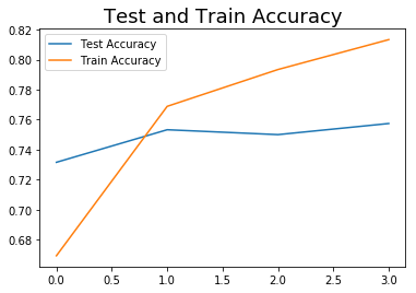
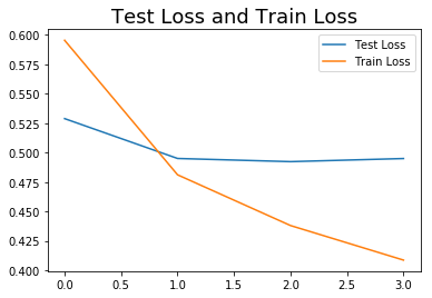
Results: Alas, after tweaking with the model several times, the best accuracy score was just shy of 75%, which is the best performance I got from the other classifying algorithms (specifically Passive Aggressive Classifier) which I had previously used.
You can see that it took only 4 epochs to converge, and EarlyStopping stopped it then.
plt.plot(history.history['val_acc'], label='Test Accuracy')
plt.plot(history.history['acc'], label='Train Accuracy')
plt.title("Test and Train Accuracy", fontsize=18)
plt.legend();
plt.plot(history.history['val_loss'], label="Test Loss")
plt.plot(history.history['loss'], label="Train Loss")
plt.title("Test Loss and Train Loss", fontsize=18)
plt.legend();
Try FFNN Model with TfIdf Vectorizer
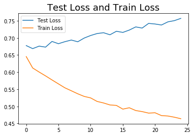
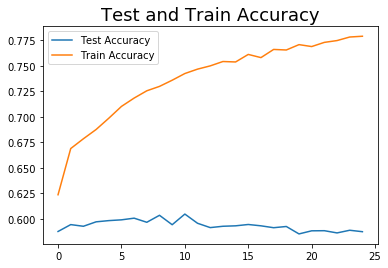
I (admittedlly quite quickly) put this together to see if a Feed Forward Neural Network would perform any differently. I suspected it wouldn’t, but as practice it was worth a shot. I vectorized the words with TdIdf and ran it through a FFNN, using this template on Kaggle as a template. After a few runs, it was clear this was not performing nearly as well as the RNN and was overfitting heavily on the training set. I adjusted the Dropout but the best score after a few tweaks was still 58% accuracy, and the model was still overfitting heavily, and failed to converge.
X = text['combined']
y = text['yes_right']
X_train, X_test, y_train, y_test = train_test_split(X, y, random_state=24, stratify=y)

X_train = [my_preprocessor(n, stop_grams=stop_grams) for n in X_train]
X_test = [my_preprocessor(n, stop_grams=stop_grams) for n in X_test]
from sklearn.feature_extraction.text import TfidfVectorizer

tf = TfidfVectorizer(max_features=200)

tfidf_mat = tf.fit_transform(X_train).toarray()
tfidf_mat_test = tf.fit_transform(X_test).toarray()
print(type(tfidf_mat),tfidf_mat.shape)  # 5572 documents, TfIdf 200 dimension
<class 'numpy.ndarray'> (27640, 200)
model = Sequential()
model.add(Dense(64,input_shape=(200,)))
model.add(Dropout(0.4))
model.add(Activation('relu'))
model.add(Dense(64))
model.add(Dropout(0.4))
model.add(Activation('relu'))
model.add(Dense(1))
model.add(Activation('sigmoid'))
model.summary()
model.compile(loss='binary_crossentropy',
              optimizer='adam',
              metrics=['acc'])
_________________________________________________________________
Layer (type)                 Output Shape              Param #
=================================================================
dense_4 (Dense)              (None, 64)                12864
_________________________________________________________________
dropout_3 (Dropout)          (None, 64)                0
_________________________________________________________________
activation_4 (Activation)    (None, 64)                0
_________________________________________________________________
dense_5 (Dense)              (None, 64)                4160
_________________________________________________________________
dropout_4 (Dropout)          (None, 64)                0
_________________________________________________________________
activation_5 (Activation)    (None, 64)                0
_________________________________________________________________
dense_6 (Dense)              (None, 1)                 65
_________________________________________________________________
activation_6 (Activation)    (None, 1)                 0
=================================================================
Total params: 17,089
Trainable params: 17,089
Non-trainable params: 0
_________________________________________________________________
history = model.fit(tfidf_mat,y_train,batch_size=32,epochs=25,validation_data=(tfidf_mat_test, y_test))
Train on 27640 samples, validate on 9214 samples
Epoch 1/25
27640/27640 [==============================] - 3s 110us/step - loss: 0.6455 - acc: 0.6237 - val_loss: 0.6776 - val_acc: 0.5877
Epoch 2/25
27640/27640 [==============================] - 3s 104us/step - loss: 0.6122 - acc: 0.6689 - val_loss: 0.6687 - val_acc: 0.5944
Epoch 3/25
27640/27640 [==============================] - 3s 103us/step - loss: 0.6004 - acc: 0.6785 - val_loss: 0.6760 - val_acc: 0.5928
Epoch 4/25
27640/27640 [==============================] - 3s 103us/step - loss: 0.5892 - acc: 0.6875 - val_loss: 0.6731 - val_acc: 0.5971
Epoch 5/25
27640/27640 [==============================] - 3s 104us/step - loss: 0.5773 - acc: 0.6986 - val_loss: 0.6897 - val_acc: 0.5983
Epoch 6/25
27640/27640 [==============================] - 3s 100us/step - loss: 0.5658 - acc: 0.7101 - val_loss: 0.6831 - val_acc: 0.5991
Epoch 7/25
27640/27640 [==============================] - 3s 96us/step - loss: 0.5543 - acc: 0.7183 - val_loss: 0.6890 - val_acc: 0.6007
Epoch 8/25
27640/27640 [==============================] - 3s 97us/step - loss: 0.5457 - acc: 0.7254 - val_loss: 0.6938 - val_acc: 0.5967
Epoch 9/25
27640/27640 [==============================] - 3s 101us/step - loss: 0.5369 - acc: 0.7297 - val_loss: 0.6887 - val_acc: 0.6035
Epoch 10/25
27640/27640 [==============================] - 3s 97us/step - loss: 0.5292 - acc: 0.7358 - val_loss: 0.6996 - val_acc: 0.5943
Epoch 11/25
27640/27640 [==============================] - 3s 95us/step - loss: 0.5249 - acc: 0.7423 - val_loss: 0.7070 - val_acc: 0.6047
Epoch 12/25
27640/27640 [==============================] - 3s 97us/step - loss: 0.5146 - acc: 0.7466 - val_loss: 0.7127 - val_acc: 0.5957
Epoch 13/25
27640/27640 [==============================] - 3s 101us/step - loss: 0.5101 - acc: 0.7498 - val_loss: 0.7152 - val_acc: 0.5915
Epoch 14/25
27640/27640 [==============================] - 3s 102us/step - loss: 0.5043 - acc: 0.7541 - val_loss: 0.7092 - val_acc: 0.5928
Epoch 15/25
27640/27640 [==============================] - 3s 96us/step - loss: 0.5030 - acc: 0.7537 - val_loss: 0.7194 - val_acc: 0.5932
Epoch 16/25
27640/27640 [==============================] - 3s 96us/step - loss: 0.4921 - acc: 0.7610 - val_loss: 0.7161 - val_acc: 0.5945
Epoch 17/25
27640/27640 [==============================] - 3s 96us/step - loss: 0.4961 - acc: 0.7579 - val_loss: 0.7229 - val_acc: 0.5932
Epoch 18/25
27640/27640 [==============================] - 3s 96us/step - loss: 0.4880 - acc: 0.7659 - val_loss: 0.7321 - val_acc: 0.5914
Epoch 19/25
27640/27640 [==============================] - 3s 97us/step - loss: 0.4849 - acc: 0.7654 - val_loss: 0.7287 - val_acc: 0.5926
Epoch 20/25
27640/27640 [==============================] - 3s 97us/step - loss: 0.4805 - acc: 0.7706 - val_loss: 0.7424 - val_acc: 0.5853
Epoch 21/25
27640/27640 [==============================] - 3s 95us/step - loss: 0.4815 - acc: 0.7687 - val_loss: 0.7406 - val_acc: 0.5883
Epoch 22/25
27640/27640 [==============================] - 3s 96us/step - loss: 0.4732 - acc: 0.7728 - val_loss: 0.7377 - val_acc: 0.5885
Epoch 23/25
27640/27640 [==============================] - 3s 97us/step - loss: 0.4720 - acc: 0.7746 - val_loss: 0.7469 - val_acc: 0.5863
Epoch 24/25
27640/27640 [==============================] - 3s 97us/step - loss: 0.4685 - acc: 0.7781 - val_loss: 0.7504 - val_acc: 0.5889
Epoch 25/25
27640/27640 [==============================] - 3s 101us/step - loss: 0.4642 - acc: 0.7788 - val_loss: 0.7570 - val_acc: 0.5875
accr = model.evaluate(tfidf_mat_test, y_test)
print("Test accuracy:", accr[1]) # Crap
9214/9214 [==============================] - 0s 26us/step
Test accuracy: 0.587475580612
plt.plot(history.history['val_acc'], label='Test Accuracy')
plt.plot(history.history['acc'], label='Train Accuracy')
plt.title("Test and Train Accuracy", fontsize=18)
plt.legend();
plt.plot(history.history['val_loss'], label="Test Loss")
plt.plot(history.history['loss'], label="Train Loss")
plt.title("Test Loss and Train Loss", fontsize=18)
plt.legend();