
Capstone Part 2 - Classifying Political News Media Text with Natural Language Processing
Now for the modeling and evaluation part of the project. Again, this was an iterative process where, using various models, I found the strongest features, checked for source giveaways or noise, and then went back and adjusted the custom list of stop words and stop-grams.
I first looked at only title and description to evaluate feature importances, and then did the same for only the numerical features created with feature engineering. Unsurprisingly, the numerical features did not have a great accuracy score, but 65% is still 12% better than the baseline. With text data, TfIdf gave me a better score with around 73.8% accuracy, an improvement of 22% from the baseline. Given this, I hoped a combination of both features in a Pipeline using FeatureUnion will improve my score upon that.
The full repo can be found here.
# Load in cleaned .csv files
text = pd.read_csv('./datasets/text2.csv').drop('Unnamed: 0', axis=1)
df = pd.read_csv('./datasets/df2.csv').drop('Unnamed: 0', axis=1)
Text Features Only
Simple CountVectorizer
# For text data only
X = text['combined']
y = text['yes_right']
X_train, X_test, y_train, y_test = train_test_split(X, y, random_state=42, stratify=y)
cvec = CountVectorizer(preprocessor=my_preprocessor,
                       strip_accents='unicode',
                       ngram_range=(1,4),
                       stop_words=cust_stop_words,
                       min_df=5)
cvec.fit(X_train, y_train);
X_feats = pd.DataFrame(cvec.transform(X_train).todense(),
                       columns=cvec.get_feature_names()).sum(axis=0)
X_feats.sort_values(ascending = False).head(15)
# Most common n-grams
trump              11671
president           5052
new                 3763
house               2301
donald              2249
donald trump        2200
says                2080
north               1980
president trump     1803
said                1789
white               1612
korea               1497
kim                 1429
people              1420
news                1360
dtype: int64
cv_train = cvec.transform(X_train).todense()
cv_test = cvec.transform(X_test).todense()
lr = LogisticRegression(random_state=42)
lr.fit(cv_train, y_train);
lr.score(cv_train, y_train), lr.score(cv_test, y_test)
(0.96280752532561509, 0.76492294334708055)
cross_val_score(lr, cv_test, y_test, scoring='accuracy', cv=7).mean()
0.72845753667711011
print(classification_report(y_test, lr.predict(cv_test)))
             precision    recall  f1-score   support

          0       0.77      0.81      0.79      4927
          1       0.76      0.71      0.74      4287

avg / total       0.76      0.76      0.76      9214
print(confusion_matrix(y_test, lr.predict(cv_test)))
# Getting a lot of false negatives.
# Model is predicting article is not right wing when it actually is
[[3982  945]
 [1223 3064]]
cfs = lr.coef_[0]
fts = cvec.get_feature_names()

pd.DataFrame(
    list(zip(fts, np.abs(cfs), cfs)),
    columns=['feat','abs','coef']).sort_values('abs',ascending=False).head(15)
# Still some noise to correct, but looking better than previous dead giveaways of source
| feat | abs | coef | |
|---|---|---|---|
| 10635 | joins discuss | 2.848528 | -2.848528 |
| 7762 | fmr | 2.781032 | -2.781032 |
| 5441 | delingpole | 2.498305 | 2.498305 |
| 13927 | nolte | 2.408937 | 2.408937 |
| 22395 | visit post | 2.293419 | 2.293419 |
| 2862 | broadcast | 2.266196 | 2.266196 |
| 21829 | tucker | 2.243125 | 2.243125 |
| 8433 | goodnewsruhles | 2.142707 | -2.142707 |
| 20839 | times local | 2.113027 | 2.113027 |
| 10032 | insight | 2.103617 | 2.103617 |
| 11807 | links | 1.954393 | 1.954393 |
| 14067 | nr | 1.931093 | 1.931093 |
| 11699 | lgbtq | 1.869136 | -1.869136 |
| 16254 | queer | 1.822175 | -1.822175 |
| 2405 | big question | 1.811977 | -1.811977 |
Passive Aggressive Classifier on Same CountVectorized data:
pac = PassiveAggressiveClassifier(C=0.5, random_state=42)
pac.fit(cv_train, y_train)
pac.score(cv_train, y_train)
0.9154486251808972
pac.score(cv_test, y_test)
0.74701541133058391
cross_val_score(pac, cv_test, y_test, scoring='accuracy', cv=7).mean()
0.70696935242130721
TfIdf Vectorizer
TfIdf’s strongest features were far less noisy than those of Count Vectorizer, meaning it’s doing its job! However, though the TfIdf model had a better accuracy score, it was predicting more false negatives than the Count Vectorizer model. Recall for the positive class was only 0.64.
tf = TfidfVectorizer(strip_accents='unicode', preprocessor=my_preprocessor,
                     ngram_range=(2,4), stop_words=cust_stop_words, min_df=2)
tf.fit(X_train, y_train)
tf_train = tf.transform(X_train)
tf_test = tf.transform(X_test)
lr = LogisticRegression(random_state=42)
parameters = {
    'penalty': ['l2','l1'],
    'C': [1.0,0.6]}

grid = GridSearchCV(lr, parameters, scoring='accuracy')
grid.fit(tf_train, y_train)
grid.score(tf_train, y_train), grid.score(tf_test, y_test)
(0.92243125904486256, 0.73855003255914908)
grid.best_params_
{'C': 1.0, 'penalty': 'l2'}
print(classification_report(y_test, grid.predict(tf_test)))
             precision    recall  f1-score   support

          0       0.72      0.82      0.77      4927
          1       0.76      0.64      0.69      4287

avg / total       0.74      0.74      0.74      9214
print(confusion_matrix(y_test, grid.predict(tf_test)))
# More false negatives but fewer false positives
[[4064  863]
 [1546 2741]]
fts = tf.get_feature_names()
cfs = grid.best_estimator_.coef_[0]

pd.DataFrame(list(zip(fts, np.abs(cfs), cfs)),
             columns=['feat','abs','coef']).sort_values('abs',ascending=False).head(15)
# Much, much less noise than CountVectorizer
| feat | abs | coef | |
|---|---|---|---|
| 47483 | michael cohen | 4.370050 | -4.370050 |
| 38742 | joins discuss | 4.056380 | -4.056380 |
| 35238 | ig report | 3.414464 | 3.414464 |
| 77969 | times local | 3.195757 | 3.195757 |
| 76722 | tel aviv | 3.082122 | 3.082122 |
| 66101 | rudy giuliani | 3.045239 | -3.045239 |
| 58979 | president trump | 3.043469 | 3.043469 |
| 31829 | gun control | 2.961285 | 2.961285 |
| 50591 | need know | 2.901651 | -2.901651 |
| 57161 | police say | 2.885630 | 2.885630 |
| 54632 | panel discusses | 2.842759 | -2.842759 |
| 13061 | charles krauthammer | 2.817736 | 2.817736 |
| 66061 | royal wedding | 2.807622 | -2.807622 |
| 43058 | left wing | 2.781428 | 2.781428 |
| 28885 | free speech | 2.753408 | 2.753408 |
text[text['combined'].str.contains('IG report')]['source'].unique()
array(['Breitbart', 'CNN', 'Fox News', 'National Review', 'Infowars',
       'MSNBC'], dtype=object)
Look at Numerical Features Only
I didn’t expect for this model to work all that well, but I wanted to see the most important features from the non-text data.
X = df[[col for col in df.columns if col != 'yes_right']]
y = df['yes_right']
X_train, X_test, y_train, y_test = train_test_split(X, y, random_state=42, stratify=y)
pipe = Pipeline([
#     ('poly', PolynomialFeatures(interaction_only=True)),
    ('model', LogisticRegression())
])

pipe.fit(X_train, y_train);
pipe.score(X_train, y_train), pipe.score(X_test, y_test)
(0.6296671490593343, 0.63338398089863257)
pd.DataFrame(list(zip(list(pipe.steps[0][1].coef_[0]),
                      np.abs(list(pipe.steps[0][1].coef_[0])), X.columns)),
             columns=['coef','coef_abs','feat']).sort_values('coef_abs', ascending=False).head(10)
| coef | coef_abs | feat | |
|---|---|---|---|
| 24 | -3.542671 | 3.542671 | PRP$_title |
| 55 | 3.161655 | 3.161655 | NNPS_desc |
| 42 | -3.045602 | 3.045602 | CC_desc |
| 6 | 2.939313 | 2.939313 | avg_word_len_title |
| 43 | 2.722251 | 2.722251 | CD_desc |
| 59 | -2.410286 | 2.410286 | PRP_desc |
| 60 | -2.396420 | 2.396420 | PRP$_desc |
| 71 | 1.986782 | 1.986782 | VBN_desc |
| 77 | -1.864823 | 1.864823 | WRB_desc |
| 44 | -1.799065 | 1.799065 | DT_desc |
Again, for reference, part of speech tag descriptions can be found here. PRP$ is possessive pronoun, NNPS is plural proper noun, and CC is conjunction.
It is interesting to note that using a possessive pronoun has a negative correlation with being right wing. This includes plural possessive pronouns, such as in “Our Revolution”.
Pipeline (Combining Text and Numerical Features)
In the Pipeline, four different models gave me around the same best accuracy scores: Passive Aggressive Classifier, Stochastic Gradient Descent Classifier, Logistic Regression, and Multinomial Naive Bayes Classifier. I decided to stick with Passive Aggressive Classifier as it had a slight edge on the others (not just because I love the name). There were a lot of different parameters to tune, in the model as well as in the Vectorizer, and I could spend a lot more time playing with this.
The Passive Aggressive Classifier works similarly to the Perceptron model, however it has the C parameter for regularization. It works very well for NLP and large datasets as it is very fast; it sees an example, updates the weights, and then discards the example. The passive aspect is that if the product is okay, the model does nothing. The aggressive aspect is that, if the product is not okay, by using the hinge loss function as the learning rate, it adjusts the weights just enough so the dot product is exactly +1. A great video explaining the workings of this algorithm can be found here.
# For Pipeline:
X = pd.concat([text['combined'], df[[col for col in df.columns if col != 'yes_right']]], axis=1)
y = df['yes_right']
num_cols = [col for col in X.columns if col != 'combined']
X_train, X_test, y_train, y_test = train_test_split(X, y, random_state=42, stratify=y)
# Function for FeatureUnion to extract data
class DfExtract(BaseEstimator, TransformerMixin):
    def __init__(self, column):
        self.column = column
    def fit(self, X, y=None):
        return self
    def transform(self, X, y=None):
        if len(self.column) > 1:
            return pd.DataFrame(X[self.column])
        else:
            return pd.Series(X[self.column[0]])
    def get_feature_names(self):
        return X.columns.tolist()
text_pipe = Pipeline([
            ('ext', DfExtract(['combined'])),
            ('tf', TfidfVectorizer(preprocessor=my_preprocessor,
                                   strip_accents='unicode',
                                   stop_words=cust_stop_words, min_df=2,
                                   ngram_range=(2,4), use_idf=True, binary=False)
            ),
#             ('lda', TruncatedSVD(n_components=500))
        ])

num_pipe = Pipeline([
            ('ext', DfExtract(num_cols)),
#             ('poly', PolynomialFeatures(interaction_only=True))
            ])
feat_union = FeatureUnion([('text', text_pipe),('numerical', num_pipe)],
                          transformer_weights={'text': 2, 'numerical': 1})
pipe = Pipeline([
    ('features', feat_union),
#     ('lda', TruncatedSVD(n_components=100)),
#     ('lr', LogisticRegression(random_state=42)),
    ('pac', PassiveAggressiveClassifier(fit_intercept=True, random_state=42))
#     ('mnb', MultinomialNB())
#     ('sgdc', SGDClassifier(random_state=42))
])
params = {
#     'lr__penalty': ['l1','l2'],
#     'lr__C': [0.33, 0.5, 0.75, 1.0],
    'pac__C': [0.25, 0.35, 0.45, 0.5, 0.65, 1],
    'pac__loss': ['hinge','squared_hinge'],
    'pac__average': [True, False]
#     'mnb__alpha': [0.001, 0.01, 0.025, 0.05, 0.1, 0.15, 0.2, 0.25]
#     'sgdc__loss': ['log','perceptron'],
#     'sgdc__penalty': ['l2','elasticnet'],
#     'sgdc__alpha': [0.00001, 0.0001, 0.001]
}

gs = GridSearchCV(pipe, params, scoring='accuracy')
gs.fit(X_train, y_train);
gs.score(X_train, y_train)
0.98136758321273521
gs.score(X_test, y_test)
0.75200781419578899
gs.best_params_
{'pac__C': 0.25, 'pac__average': True, 'pac__loss': 'hinge'}
Evaluate Model
Evaluating the first models that looked at text data and numerical data separately, it is clear that TfIdf Vectorizer did its job. The inverse document frequency weighting factor greatly reduced the amount of noise in the strongest coefficients compared to the Count Vectorizer model. Furthermore, as accuracy increased with TfIdf, the amount of false positives increased and false negatives increased. The recall score for the positive class was only 64%. This makes sense as there are several thousand more not right wing sources than right wing sources. I hoped that I could account for this in the Pipeline model that balances text data with numerical data.
In the main Pipeline model, the 75.2% accuracy score isn’t as good as I had hoped for, but it is important to note that this score declined significantly the more I evaluated the model results and appropriately cleaned the data more, reducing noise and source giveaways. This helped to reduce overfitting; previously the train set score was a perfect 1.0. After cleaning the data more, the model will likely perform better on other political news media text outside of the data I have collected. For example, “Fast Facts” was previously a bi-gram with a very strong negative coefficient. This ended up being a giveaway for CNN. Removing it didn’t help my accuracy score, but improved the general performance of the model as it is intended to function.
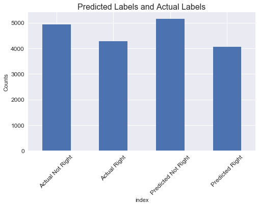
Furthermore, compared to the models I ran on the text data and numerical data separately, the Pipeline using the Passive Aggressive Classifier accounted for the previous issue of having many false positives. Accuracy, recall, precision, and F1 scores were all 75%, as there were about the same about of false positives as false negatives. Although there are no ethical considerations to consider when classifying political text—misclassifying a right wing article as not right wing isn’t any better or worse than misclassifying a not right wing article as right wing—it is an indication that the model is performing better overall when the errors are more balanced because the classes are slightly unbalanced in favor of not right wing sources.
y_counts = pd.DataFrame(y_test)['yes_right'].value_counts()
yhat_counts = pd.DataFrame(gs.predict(X_test))[0].value_counts()
pred_df = pd.DataFrame(pd.concat([y_counts, yhat_counts], axis=0))
pred_df['index']=['Actual Not Right','Actual Right','Predicted Not Right', 'Predicted Right']
pred_df.set_index('index', inplace=True)
pred_df.plot(kind='bar', rot=45, fontsize=12, figsize=(8,5), legend=False, use_index=True)
plt.title("Predicted Labels and Actual Labels", fontsize=16)
plt.ylabel('Counts');
print(classification_report(y_test, gs.predict(X_test)))
             precision    recall  f1-score   support

          0       0.76      0.79      0.77      4927
          1       0.75      0.71      0.73      4287

avg / total       0.75      0.75      0.75      9214
import itertools
# From ScikitLearn's documentation:
def plot_confusion_matrix(cm, classes,
                          normalize=False,
                          title='Confusion matrix',
                          cmap="Blues"):
    """
    This function prints and plots the confusion matrix.
    Normalization can be applied by setting `normalize=True`.
    """
    if normalize:
        cm = cm.astype('float') / cm.sum(axis=1)[:, np.newaxis]
        print("Normalized confusion matrix")
    else:
        print('Confusion matrix, without normalization')

    print(cm)

    plt.imshow(cm, interpolation='nearest', cmap=cmap)
    plt.title(title, fontsize=18)
    plt.colorbar()
    tick_marks = np.arange(len(classes))
    plt.xticks(tick_marks, classes, rotation=45)
    plt.yticks(tick_marks, classes)

    fmt = '.2f' if normalize else 'd'
    thresh = cm.max() / 2.
    for i, j in itertools.product(range(cm.shape[0]), range(cm.shape[1])):
        plt.text(j, i, format(cm[i, j], fmt),
                 horizontalalignment="center",
                 color="white" if cm[i, j] > thresh else "black")

    plt.tight_layout()
    plt.ylabel('True label', fontsize=16)
    plt.xlabel('Predicted label', fontsize=16)
np.set_printoptions(precision=2)
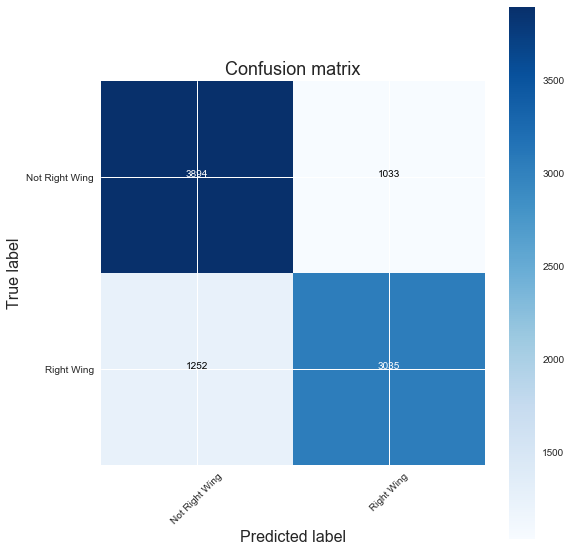
plt.figure(figsize=(8,8))
plot_confusion_matrix(confusion_matrix(y_test, gs.predict(X_test)),
classes=['Not Right Wing','Right Wing'],
title='Confusion matrix')
plt.show()
Confusion matrix, without normalization
[[3894 1033]
 [1252 3035]]
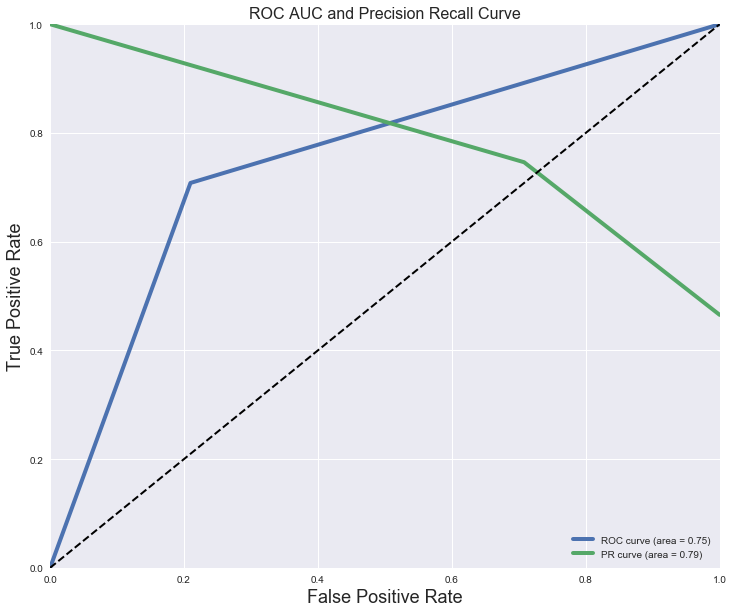
# ROC AUC Curve looks a bit silly without predict_proba
y_hat = gs.predict(X_test) # Model's predictions

# For class 1, find the area under the curve
false_pos, true_pos, _ = roc_curve(y_test, y_hat)
ROC_AUC = auc(false_pos, true_pos)
prec, rec, _ = precision_recall_curve(y_test, y_hat)
PR_AUC = auc(rec, prec)

# Plot of a ROC curve for class 1 (has_cancer)
plt.figure(figsize=[12,10])
plt.plot(false_pos, true_pos, label='ROC curve (area = %0.2f)' % ROC_AUC, linewidth=4)
plt.plot(rec, prec, label='PR curve (area = %0.2f)' % PR_AUC, linewidth=4)
plt.plot([0, 1], [0, 1], 'k--', linewidth=2)
plt.xlim([0.0, 1.0])
plt.ylim([0.0, 1.0])
plt.xlabel('False Positive Rate', fontsize=18)
plt.ylabel('True Positive Rate', fontsize=18)
plt.title('ROC AUC and Precision Recall Curve', fontsize=16)
plt.legend(loc="lower right")
plt.show()
Interpret Results
Interpreting this model has become less and less challenging the more the data has been appropriately cleaned. However, by looking at the strongest coefficients, it is clear there is still some work to do. “Gerber baby” had not appeared in the top strongest coefficients until the most recent iteration of running the model. However, we are starting to see some n-grams that make sense, such as “far left anti” being correlated with right wing articles. As this model continues to be tuned, it will provide more insight into what kind of language is used differently based on the kind of news source the language is found in. A high amount of possessive pronouns in the article title has a strong correlation with being not right wing, for example. Furthermore, the word cloud displays words ignored by the model because they either occurred in too many documents, occurred in to few documents, or were cut off by feature selection. It is what you’d expect to see, but a fun graphic nevertheless.
Getting Feature Importances
feature_names = text_pipe.fit(X_train, y_train).steps[1][1].get_feature_names()
feature_names.extend(num_pipe.fit(X_train, y_train).steps[0][1].get_feature_names())
pipe_coefs = list(gs.best_estimator_.steps[1][1].coef_[0])
feature_names.remove(feature_names[0])
importances = pd.DataFrame(list(zip(feature_names, pipe_coefs, np.abs(pipe_coefs))),
                          columns=['feature','coef','abs_coef'])
importances.sort_values('abs_coef', ascending=False).head(15)
| feature | coef | abs_coef | |
|---|---|---|---|
| 38734 | joins discuss allegations | -2.570853 | 2.570853 |
| 77954 | times local 05 | 2.363183 | 2.363183 |
| 88195 | PRP$_title | -2.001645 | 2.001645 |
| 51772 | news news brexit | 1.942494 | 1.942494 |
| 26514 | far left anti | 1.765146 | 1.765146 |
| 35235 | ig report calls | 1.737069 | 1.737069 |
| 54622 | panel discusses latest | -1.696134 | 1.696134 |
| 43049 | left wing activist | 1.685441 | 1.685441 |
| 13060 | charles krauthammer beloved | 1.656427 | 1.656427 |
| 83728 | visit president | 1.601330 | 1.601330 |
| 88177 | avg_word_len_title | 1.589872 | 1.589872 |
| 88213 | CC_desc | -1.545891 | 1.545891 |
| 29947 | gerber baby | 1.495070 | 1.495070 |
| 76708 | tel aviv capital | 1.463338 | 1.463338 |
| 66089 | rudy giuliani booed | -1.460225 | 1.460225 |
Still some noise in here. Apparently there was a story about the original Gerber baby meeting the current Gerber baby that was covered in multiple outlets. This ideally shouldn’t predict whether an article is right wing or not. Some of this is straddling the line between discovering hidden statistical correlations (machine learning!) and just plain old noise.
text[text['combined'].str.contains('Gerber baby')]['source'].unique()
array(['National Review', 'Huffington Post'], dtype=object)
feat_imports = importances.sort_values('abs_coef', ascending=True).tail(15)
feat_imports['sign'] = feat_imports['coef'].map(lambda x: 'Negative' if x < 0 else 'Positive')
feat_imports.set_index('feature', inplace=True)

feat_imports['coef'].plot(kind='barh', figsize=(12,6),
                  title='Strongest Coefficients (Absolute Value)',
                  fontsize=14, legend=False, color='navy')
plt.xlabel('Coefficient')
plt.title('Top 15 Strongest Coefficients', fontsize=18);
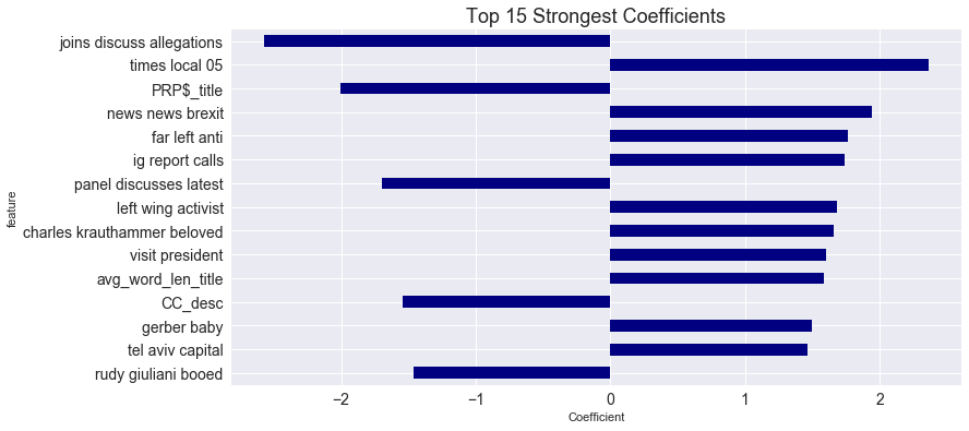
PRP$_title means possesive pronoun in title and CC_desc is conjunction in description.
# Plot words ignored by model
text_pipe.fit(X_train, y_train)
ignored_text = text_pipe.steps[1][1].stop_words_
plt.figure(figsize=(15,8))
wordcloud = WordCloud(font_path='/Library/Fonts/Verdana.ttf',
                      width=2000, height=1000,
                      relative_scaling = 1.0,
                      background_color='white',
                      colormap='Dark2'

).generate(' '.join(ignored_text))
plt.imshow(wordcloud)
plt.title("Words Ignored by Model", fontsize=28)
plt.axis("off")
plt.show()
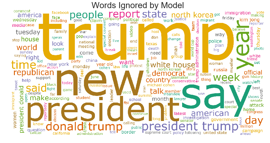
These are all of TfIdf’s stop words: the words ignored by the model because they either occurred in too many documents, occurred in too few documents, or were cut off by feature selection.
Next Steps
There is clearly a lot of work that can be done with this project to improve on it. Given that the data is fairly time-specific (a 5-6 month period), I would like to gather more article data from other time periods, both from the past and in the future. I would also like to continue creating more features from the text using other NLP tools. Likewise, I would like to implement a Recurrent Neural Network to see if accuracy is improved. Nevertheless, it was a fun project to see what I could do with this dataset, and the project can function as a springboard to more bigger and complex NLP projects. This project was a very enjoyable learning experience to work on and will certainly continue to be as I keep playing with it.