
Capstone Part 1 - Classifying Political News Media Text with Natural Language Processing
For my final capstone project as part of the Data Science Immersive program at General Assembly NYC, I decided to create a political text classification model using Natural Language Processing. As with all data science projects, this was a non-linear, iterative process that required extensive data cleaning. I learned a great deal about NLP in the process, and I look forward to further projects on this topic. The full repo for this project can be found here.
Purpose
In 2018, I don’t think I need to remind anyone of the current news media landscape in the United States. Needless to say, the media culture is extremely polarized and the societal effects of how people source their information is becoming increasingly evident. It hasn’t always been this way, and it is important to be able to know what kind of source a piece of political news text is coming from before deciding what to do with it. Political Science is often defined as the study of power. In the era of Trump, the power of language is increasingly relevant and important. In this project, I aim to build a model that predicts whether or not political media text is right wing or not right wing. I could have chosen to call these labels “right” and “left”, but I chose more of a “one vs. rest” terminology to reflect the fact that the political spectrum isn’t as simple as Right and Left. This website has a great “media bias chart” for visualization. There is more to say about far right news media entering the mainstream, but we can save that for another day. Furthermore, this project is a stepping stone to future projects using multi class targets that more accurately reflect the kinds of political news media that are out there. Likewise, it is a stepping stone to more intimidating and complex projects that tackle social media language as well.
Gathering and Load Data
I collected data for 36,854 unique articles from a variety of right wing and not right wing sources. The features collected were title, description, date posted, url, author, and source. Choosing obviously partisan sources, I labeled whether they are right wing or not based on the source. Therefore, since I would only be starting with title and description as features, a challenge I faced is making sure that any giveaway of the source is removed from an article’s text features. All of my data was scraped from News API except for Infowars and Democracy Now, for which I used BeautifulSoup to scrape article information from their respective RSS feeds.
My right wing sources included:
- Fox News
- Breitbart News
- National Review
- Infowars
Not right wing sources:
- MSNBC
- Huffington Post
- Vice News
- CNN
- Democracy Now!
I scraped the data in separate notebooks and then loaded in all of the individual .csv files into my main notebook. The notebooks for this data collection process can be found in the main folder of the GitHub repo.
Clean Data
The initial data cleaning was quite simple and straightforward compared to the iterative process of removing noisy n-grams that would come once I began exploring and modeling. I dropped all of the rows with missing titles or descriptions, as those are the only features I would start with in my model.
# Check for missing values
text.isna().sum()
author         9466
description      69
publishedAt       0
source            0
title             1
url               0
yes_right         0
dtype: int64
# Dropped all rows with missing text, as that is all I will be using as features
text.dropna(subset=['description','title'], inplace=True)
# It's okay if there is no author
text.fillna('no_author', inplace=True)
text.shape
(36854, 7)
text.yes_right.value_counts()[0]/len(text.yes_right)
# Baseline accuracy is 53.5%, almost a 50/50 split in target
# There are a bit more not right sources than right
0.53470450968687255
It’s barely worth including Infowars and Democracy Now in the model as it would have taken quite a long time to gather a comparable amount of articles as those from News API by scraping from an RSS feed. However, I got as many articles as I could over a week’s time.
text.source.value_counts()
# Democracy Now and Infowars don't produce quite as much content...
fox news           6381
national review    5348
huffington post    4950
msnbc              4950
vice news          4949
breitbart          4948
cnn                4776
infowars            471
democracy now        81
Name: source, dtype: int64
Removing Source Giveaways from the Title and Description
There was a multi-step process to remove source giveaways from the articles’ text features. Here I create a function to use in the .apply() function to remove any mention of any source from all of the title and description text, as well as remove that specific article’s author from the text. This cleaned up a lot of source giveaways, but there was still much that slipped through the cracks.
# Many CNN articles had "CNN" after the author's name
text['author'] = [a.replace(', CNN', '') for a in text['author']]
def remove_source_info(row):
    sources = ['Breitbart', 'CNN', 'Fox News', 'National Review', 'Vice News',
               'Democracy Now', 'Infowars', 'MSNBC', 'Huffington Post']
    for source in sources:
        row['description'] = row['description'].replace(source, '')
        row['title'] = row['title'].replace(source, '')
    row['title'] = row['title'].replace(row['author'], '')
    row['description'] = row['description'].replace(row['author'], '')
    return row
text = text.apply(remove_source_info, axis=1)
text.query("source=='Fox News'").head()
| author | description | publishedAt | source | title | url | yes_right | |
|---|---|---|---|---|---|---|---|
| 9724 | no_author | Judge Napolitano and Marie Harf discuss the Tr... | 2018-06-20T18:51:36Z | Fox News | Freedom Watch: Napolitano and Harf dig in on i... | http://video.foxnews.com/v/5799861947001/ | 1 |
| 9725 | no_author | Find out where and who caught a rare cotton ca... | 2018-06-20T18:50:00Z | Fox News | See it: Cotton candy-colored lobster caught | http://video.foxnews.com/v/5799865520001/ | 1 |
| 9726 | no_author | Steve Harrigan reports from outside a detentio... | 2018-06-20T18:47:58Z | Fox News | Media not given access to 'tender age' shelters | http://video.foxnews.com/v/5799862990001/ | 1 |
| 9727 | no_author | Reports: More than 2,000 children have been se... | 2018-06-20T18:47:54Z | Fox News | Critics denounce 'tender age' shelters | http://video.foxnews.com/v/5799860019001/ | 1 |
| 9728 | no_author | Nearly a year after the body of little boy was... | 2018-06-20T18:38:34Z | Fox News | ‘Little Jacob’ has been identified | http://video.foxnews.com/v/5799856889001/ | 1 |
NLP Feature Engineering
Using NLP tools from the TextBlob library, I tagged each word of the title and description with a part of speech and added the normalized value counts for each part of speech as a new feature. The meaning of those parts of speech tags can be found here. I also used TextBlob’s sentiment analysis scoring to create features for polarity (positive or negative) and subjectivity. I then took the difference between title polarity and description polarity as well as the difference between title subjectivity and description subjectivity to measure any possible discrepancy in sentiment between title and description. Additionally, I created an average title word length feature. I could have spent weeks just engineering features using NLP tools, but this seemed like a good base to start with for this project.
text['combined'] = text.title + ' ' + text.description # all text together
For creation of features, I treated title and description separately, but for modeling with TfIdf I combined the two into one document for each row.
I created a feature of average word length in the title using a RegEx tokenizer.
tokenizer = nltk.RegexpTokenizer(r'\w+')
title_tokens = [tokenizer.tokenize(w) for w in text.title]

avg_word_length = []
for title in title_tokens:
    wordlen = []
    for word in title:
        wordlen.append(len(word))
        if len(wordlen)==len(title):
            avg_word_length.append(np.sum(wordlen)/len(wordlen))

text['avg_word_len_title'] = avg_word_length
Sentiment Analysis
I used TextBlob to create polarity and subjectivity features for both the title and description.
text['title_polarity'] = [TextBlob(w).sentiment.polarity for w in text.title]

text['title_subjectivity'] = [TextBlob(w).sentiment.subjectivity for w in text.title]

text['desc_polarity'] = [TextBlob(w).sentiment.polarity for w in text.description]

text['desc_subjectivity'] = [TextBlob(w).sentiment.subjectivity for w in text.description]

text['subj_difference'] = text['title_subjectivity'] - text['desc_subjectivity']
text['polarity_difference']  = text['title_polarity'] - text['desc_polarity']
Parts of Speech Tagging
Also using TextBlob, I tagged each word with a part of speech and then took the normalized value counts for each part of speech in the document.
title_tags = [TextBlob(w.lower(), tokenizer=tokenizer).tags for w in text.title]
title_tags[0]
[('peter', 'NN'),
 ('fonda', 'NN'),
 ('lying', 'VBG'),
 ('gash', 'JJ'),
 ('kirstjen', 'NNS'),
 ('nielsen', 'VBN'),
 ('should', 'MD'),
 ('be', 'VB'),
 ('whipped', 'VBN'),
 ('naked', 'JJ'),
 ('in', 'IN'),
 ('public', 'JJ')]
tags_counts = []
for row in title_tags:
    tags = [n[1] for n in row]
    tags_counts.append(tags)
title_parts_of_speech = []
for n in tags_counts:
    foo = dict(pd.Series(n).value_counts(normalize=True))
    title_parts_of_speech.append(foo)
title_parts_of_speech = pd.DataFrame(title_parts_of_speech).fillna(0)
# A NaN value means that part of speech did not appear in the text
# Label as title parts of speech
title_parts_of_speech.columns = [str(n) + '_title' for n in title_parts_of_speech.columns]
I then followed the same process for description.
# Checking for correct length
desc_parts_of_speech.shape[0] == title_parts_of_speech.shape[0]
True
pos_tags = pd.concat([title_parts_of_speech, desc_parts_of_speech], axis=1)
# Concatenate all created features together with target
df = pd.concat([text[['title_polarity', 'title_subjectivity', 'desc_polarity',
                      'desc_subjectivity', 'subj_difference', 'polarity_difference',
                      'avg_word_len_title']], pos_tags, text.yes_right], axis=1)
df.head(3)
| title_polarity | title_subjectivity | desc_polarity | desc_subjectivity | subj_difference | polarity_difference | avg_word_len_title | CC_title | CD_title | DT_title | ... | VBD_desc | VBG_desc | VBN_desc | VBP_desc | VBZ_desc | WDT_desc | WP_desc | WP$_desc | WRB_desc | yes_right | |
|---|---|---|---|---|---|---|---|---|---|---|---|---|---|---|---|---|---|---|---|---|---|
| 0 | 0.50 | 0.233333 | 0.500000 | 0.000000 | 0.233333 | 0.000000 | 5.166667 | 0.0 | 0.0 | 0.0 | ... | 0.068182 | 0.045455 | 0.022727 | 0.0 | 0.00 | 0.0 | 0.022727 | 0.0 | 0.0 | 1 |
| 1 | 0.25 | 0.900000 | 0.250000 | 0.650000 | 0.250000 | 0.000000 | 5.750000 | 0.0 | 0.0 | 0.0 | ... | 0.000000 | 0.160000 | 0.040000 | 0.0 | 0.04 | 0.0 | 0.000000 | 0.0 | 0.0 | 1 |
| 2 | 0.40 | 0.300000 | 0.555417 | 0.666667 | -0.366667 | -0.155417 | 6.545455 | 0.0 | 0.0 | 0.0 | ... | 0.020000 | 0.060000 | 0.020000 | 0.1 | 0.04 | 0.0 | 0.000000 | 0.0 | 0.0 | 1 |
3 rows × 79 columns
Every created features is already scaled except for a few, which I just simply manually scaled.
def scaled_checker(df):
    for col in df.columns:
        if max(df[col]) > 1:
            print(col)
        if min(df[col]) < 0:
            print(col)
        else:
            pass

scaled_checker(df)
subj_difference
polarity_difference
avg_word_len_title
df['subj_difference'] = (df['subj_difference'] - min(df['subj_difference'])) \n
    /(max(df['subj_difference'])-min(df['subj_difference']))
df['polarity_difference'] = (df['polarity_difference'] - min(df['polarity_difference']))/ \n
    (max(df['polarity_difference'])-min(df['polarity_difference']))
df['avg_word_len_title'] = (df['avg_word_len_title'] - min(df['avg_word_len_title']))/ \n
    (max(df['avg_word_len_title'])-min(df['avg_word_len_title']))
scaled_checker(df) # numerical data is scaled
# Save my mostly cleaned datasets
text.to_csv('./datasets/text2.csv')
df.to_csv('./datasets/df2.csv')
Explore Data
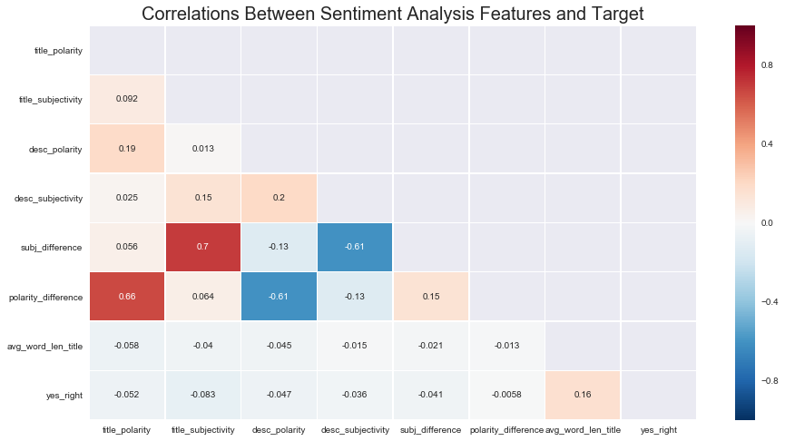
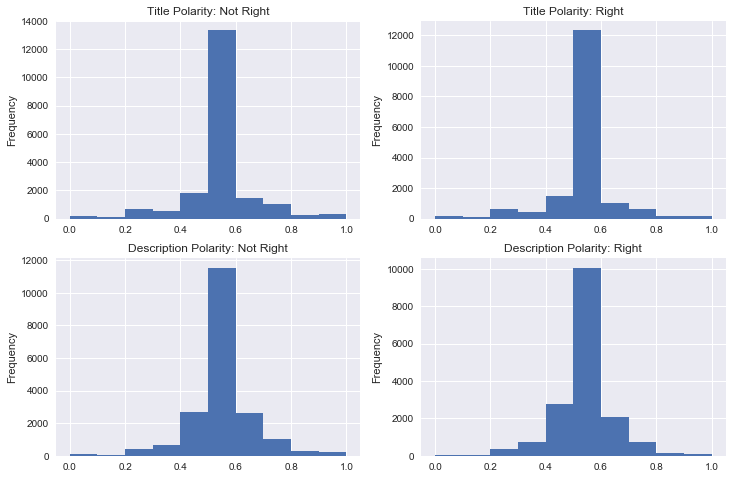
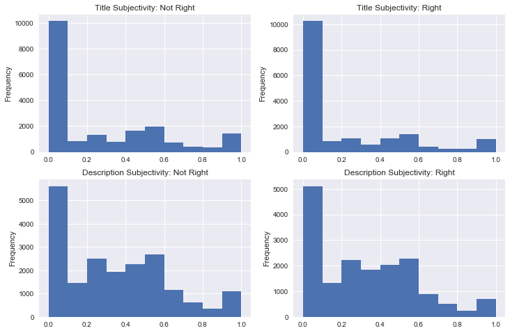
Exploring the sentiment analysis features, there is not much significant to note. Correlations between features and the target are extremely weak. All distributions had the same shape, with all of polarity having a normal distribution and all description distributions being skewed right. In other words, most text was neutral in terms of polarity and most text was more objective than subjective. One difference is that there was more subjective language in the descriptions than in the titles.
num_corrs = df[['title_polarity','title_subjectivity','desc_polarity',
                'desc_subjectivity', 'subj_difference','polarity_difference',
                'avg_word_len_title','yes_right']].corr()
mask = np.zeros_like(num_corrs, dtype=np.bool)
mask[np.triu_indices_from(mask)] = True
plt.figure(figsize=(15,8))
plt.title('Correlations Between Sentiment Analysis Features and Target', fontsize=20)
sns.heatmap(num_corrs, linewidths=0.5, mask=mask, annot=True);
# Very insignificant
# Looking at features based on target
rightwing = df[df.yes_right==1]
notrightwing = df[df.yes_right==0]
figure, ax = plt.subplots(nrows=2, ncols=2, figsize=(12, 8))

rightwing.title_polarity.plot(kind='hist', ax=ax[0,1],
                              title='Title Polarity: Right')
notrightwing.title_polarity.plot(kind='hist', ax=ax[0,0],
                                 title='Title Polarity: Not Right')
notrightwing.desc_polarity.plot(kind='hist',
                                ax=ax[1,0], title='Description Polarity: Not Right')
rightwing.desc_polarity.plot(kind='hist',
                             ax=ax[1,1], title='Description Polarity: Right');
figure, ax = plt.subplots(nrows=2, ncols=2, figsize=(12, 8))

rightwing.title_subjectivity.plot(kind='hist', ax=ax[0,1],
                                  title='Title Subjectivity: Right')
notrightwing.title_subjectivity.plot(kind='hist', ax=ax[0,0],
                                     title='Title Subjectivity: Not Right')
notrightwing.desc_subjectivity.plot(kind='hist', ax=ax[1,0],
                                    title='Description Subjectivity: Not Right')
rightwing.desc_subjectivity.plot(kind='hist', ax=ax[1,1],
                                 title='Description Subjectivity: Right');
Exploring Word Counts
In the following several sections, I used Count Vectorizer to find the highest count single-grams, bi-grams, tri-grams, and quad-grams in the titles and descriptions, sorted by both target classes. After initially looking at the counts and seeing a lot of source information and noise, I created a custom preprocessor that removes stop grams of noise and source information as well as lemmatize the text. I also created a custom group of stop words that contain source information and appended it to SciKitLearn’s list of English stop words, which I used in all of my Count Vectorizer and TfIdf models. The initial words counts demonstrated that there is much noise in the data, and TfIdf might be the best choice for a vectorizer as it will penalize terms that appear very frequently across documents. However, if some of these terms only appear frequently in only one unique source, I decided to remove them manually.
There were a couple interesting interpretations, especially as the n-grams increased, but the most common n-grams in the documents were mostly similar between left and right until the tri-gram level, when noticeable differences began to form.
Set Up Vectorizer
lemmatizer = WordNetLemmatizer()

def my_preprocessor(doc):
    stop_grams = ['national review','National Review','Fox News','Content Uploads',
                  'content uploads','fox news', 'Associated Press','associated press',
                  'Fox amp Friends','Rachel Maddow','Morning Joe','morning joe',
                  'Breitbart News', 'fast facts', 'Fast Facts','Fox &', 'Fox & Friends',
                  'Ali Velshi','Stephanie Ruhle','Raw video', '& Friends', 'Ari Melber',
                  'amp Friends', 'Content uploads', 'Geraldo Rivera']
    for stop in stop_grams:
        doc = doc.replace(stop,'')
    return lemmatizer.lemmatize(doc.lower())
cust_stop_words = ['CNN','cnn','amp','huffpost','fox','reuters','ap','vice','breitbart',
                   'nationalreview', 'www','msnbc','infowars', 'foxnews','Vice','Breitbart',
                   'National Review','Fox News','Reuters','Fast Facts','Infowars','Vice',
                   'MSNBC','www','AP','Huffpost','HuffPost','Maddow', '&', 'Ingraham', 'ingraham']
from sklearn.feature_extraction.text import ENGLISH_STOP_WORDS
original_stopwords = list(ENGLISH_STOP_WORDS)
cust_stop_words += original_stopwords
Single Grams for Title
right = text['yes_right'] == 1
notright = text['yes_right'] == 0
# Separate title and description based on target class
right_title = text[right].title
right_desc = text[right].description
notright_title = text[notright].title
notright_desc = text[notright].description
stem = PorterStemmer()
lemmatizer = WordNetLemmatizer()
def get_top_grams(df_r, df_nr, n):
    cvec = CountVectorizer(preprocessor=my_preprocessor,
                           ngram_range=(n,n), stop_words=cust_stop_words, min_df=5)
    cvec.fit(df_r)
    word_counts = pd.DataFrame(cvec.transform(df_r).todense(),
                       columns=cvec.get_feature_names())
    counts = word_counts.sum(axis=0)
    counts = pd.DataFrame(counts.sort_values(ascending = False),columns=['right']).head(15)

    cvec = CountVectorizer(preprocessor=my_preprocessor,
                           ngram_range=(n,n), stop_words=cust_stop_words, min_df=5)
    cvec.fit(df_nr)
    word_counts2 = pd.DataFrame(cvec.transform(df_nr).todense(),
                         columns=cvec.get_feature_names())
    counts2 = word_counts2.sum(axis=0)
    counts2 = pd.DataFrame(counts2.sort_values(ascending = False),columns=['not right']).head(15)
    return counts, counts2
r
| right | |
|---|---|
| trump | 2981 |
| report | 569 |
| north | 523 |
| korea | 502 |
| says | 481 |
| new | 453 |
| house | 419 |
| border | 419 |
| kim | 397 |
| summit | 390 |
| president | 386 |
| day | 375 |
| police | 366 |
| immigration | 340 |
| donald | 304 |
nr
| not right | |
|---|---|
| trump | 3872 |
| new | 1043 |
| says | 585 |
| house | 471 |
| 2018 | 430 |
| north | 414 |
| korea | 401 |
| cohen | 391 |
| mueller | 377 |
| white | 350 |
| kim | 347 |
| 18 | 339 |
| world | 338 |
| like | 333 |
| gop | 328 |
Single Grams for Description
r, nr = get_top_grams(right_desc, notright_desc, 1)
r
| right | |
|---|---|
| trump | 3830 |
| president | 3216 |
| new | 1479 |
| house | 1214 |
| said | 1205 |
| donald | 1111 |
| north | 938 |
| state | 909 |
| says | 846 |
| news | 760 |
| year | 735 |
| white | 734 |
| police | 703 |
| tuesday | 682 |
| people | 632 |
nr
| not right | |
|---|---|
| trump | 4756 |
| president | 2799 |
| new | 2052 |
| donald | 1374 |
| said | 1093 |
| house | 1039 |
| says | 840 |
| people | 831 |
| discuss | 777 |
| white | 768 |
| north | 721 |
| michael | 710 |
| news | 687 |
| day | 623 |
| year | 584 |
BiGrams for Title
r, nr = get_top_grams(right_title, notright_title, 2)
r
| right | |
|---|---|
| north korea | 417 |
| donald trump | 303 |
| white house | 230 |
| kim jong | 182 |
| president trump | 181 |
| ig report | 141 |
| supreme court | 129 |
| trump kim | 121 |
| judicial activism | 104 |
| day liberal | 104 |
| liberal judicial | 104 |
| new york | 100 |
| year old | 91 |
| kim summit | 82 |
| cartoons day | 80 |
nr
| not right | |
|---|---|
| north korea | 321 |
| white house | 247 |
| michael cohen | 196 |
| kim jong | 165 |
| donald trump | 160 |
| stormy daniels | 113 |
| world cup | 111 |
| royal wedding | 99 |
| scott pruitt | 98 |
| president trump | 96 |
| new york | 87 |
| korea summit | 86 |
| family separation | 85 |
| trump kim | 83 |
| kanye west | 77 |
BiGrams for Description
r, nr = get_top_grams(right_desc, notright_desc, 2)
r # Seeing some noise here
| right | |
|---|---|
| president trump | 1187 |
| donald trump | 1088 |
| president donald | 932 |
| white house | 621 |
| new york | 481 |
| kim jong | 474 |
| north korea | 473 |
| year old | 339 |
| united states | 314 |
| north korean | 313 |
| trump administration | 257 |
| wp com | 238 |
| content uploads | 238 |
| com com | 238 |
| wp content | 238 |
nr
| not right | |
|---|---|
| donald trump | 1352 |
| president trump | 904 |
| president donald | 673 |
| white house | 640 |
| new york | 420 |
| kim jong | 414 |
| michael cohen | 405 |
| trump administration | 401 |
| north korea | 386 |
| north korean | 254 |
| special counsel | 236 |
| robert mueller | 233 |
| rudy giuliani | 224 |
| united states | 223 |
| stormy daniels | 213 |
TriGrams for Title
r, nr = get_top_grams(right_title, notright_title, 3)
r # Mentions of MS 13 Gang and "judicial activism"
| right | |
|---|---|
| liberal judicial activism | 104 |
| day liberal judicial | 104 |
| north korea summit | 75 |
| trump kim summit | 66 |
| new york times | 27 |
| border patrol agents | 26 |
| south china sea | 26 |
| trump kim jong | 23 |
| judicial activism june | 22 |
| cartoons day march | 21 |
| judicial activism march | 20 |
| ms 13 gang | 20 |
| judicial activism april | 19 |
| cartoons day april | 19 |
| judicial activism february | 19 |
nr
# Interesting: NYT is not one of my sources
# Mentions of Stormy Daniels and immigration policy
| not right | |
|---|---|
| north korea summit | 73 |
| trump kim summit | 37 |
| family separation policy | 29 |
| trump tower meeting | 28 |
| quickly catch day | 21 |
| catch day news | 21 |
| trump legal team | 21 |
| trump north korea | 20 |
| iran nuclear deal | 20 |
| stormy daniels lawyer | 19 |
| daily horoscope june | 19 |
| trump kim jong | 18 |
| mtp daily june | 17 |
| santa fe high | 17 |
| sarah huckabee sanders | 17 |
TriGrams for Description
r, nr = get_top_grams(right_desc, notright_desc, 3)
r # For some reason "content uploads" is still appearing. Source giveaway.
# Also image noise data.
| right | |
|---|---|
| president donald trump | 926 |
| wp com com | 238 |
| wp content uploads | 238 |
| com wp content | 238 |
| com com wp | 238 |
| content uploads 2018 | 233 |
| jpg fit 1024 | 218 |
| 1024 2c597 ssl | 216 |
| fit 1024 2c597 | 216 |
| dictator kim jong | 125 |
| new york times | 118 |
| special counsel robert | 110 |
| leader kim jong | 108 |
| counsel robert mueller | 108 |
| new york city | 102 |
nr
| not right | |
|---|---|
| president donald trump | 672 |
| north korean leader | 158 |
| new york times | 155 |
| leader kim jong | 149 |
| korean leader kim | 133 |
| special counsel robert | 125 |
| counsel robert mueller | 123 |
| fbi director james | 81 |
| director james comey | 81 |
| joy reid panel | 81 |
| reid panel discuss | 74 |
| lawyer michael cohen | 69 |
| attorney general jeff | 64 |
| general jeff sessions | 64 |
| new york city | 60 |
QuadGrams for Title
r, nr = get_top_grams(right_title, notright_title, 4)
r
# Again, lost of "judicial activism" and MS 13 appears
| right | |
|---|---|
| day liberal judicial activism | 104 |
| liberal judicial activism june | 22 |
| liberal judicial activism march | 20 |
| liberal judicial activism february | 19 |
| liberal judicial activism april | 19 |
| things caught eye today | 11 |
| north korea kim jong | 9 |
| fashion notes melania trump | 9 |
| santa fe high school | 7 |
| new york attorney general | 7 |
| public sector union dues | 7 |
| ms 13 gang members | 7 |
| fashion designer kate spade | 7 |
| southern poverty law center | 7 |
| trump says north korea | 7 |
nr
| not right | |
|---|---|
| quickly catch day news | 21 |
| santa fe high school | 15 |
| trump family separation policy | 14 |
| prince harry meghan markle | 13 |
| new albums heavy rotation | 11 |
| new shows netflix stream | 10 |
| watch hulu new week | 10 |
| watch amazon prime new | 10 |
| trump north korea summit | 10 |
| amazon prime new week | 10 |
| best new shows netflix | 10 |
| shows netflix stream right | 10 |
| ranking best new shows | 10 |
| funniest tweets women week | 9 |
| 20 funniest tweets women | 9 |
QuadGrams for Description
r, nr = get_top_grams(right_desc, notright_desc, 4)
r
# Very noisy
| right | |
|---|---|
| com wp content uploads | 238 |
| com com wp content | 238 |
| wp com com wp | 238 |
| wp content uploads 2018 | 233 |
| fit 1024 2c597 ssl | 216 |
| jpg fit 1024 2c597 | 209 |
| special counsel robert mueller | 108 |
| north korean dictator kim | 94 |
| korean dictator kim jong | 94 |
| north korean leader kim | 91 |
| korean leader kim jong | 90 |
| https i0 wp com | 83 |
| i0 wp com com | 83 |
| i2 wp com com | 78 |
| https i2 wp com | 78 |
nr
# Less noise, but still source giveaways like "Chris Matthews".
| not right | |
|---|---|
| north korean leader kim | 133 |
| korean leader kim jong | 132 |
| special counsel robert mueller | 123 |
| fbi director james comey | 81 |
| joy reid panel discuss | 74 |
| attorney general jeff sessions | 63 |
| discuss political news day | 56 |
| matthews panel guests discuss | 56 |
| panel guests discuss political | 56 |
| guests discuss political news | 56 |
| chris matthews panel guests | 56 |
| mika discuss big news | 55 |
| joe mika discuss big | 55 |
| discuss big news day | 55 |
| hayes discusses day political | 55 |
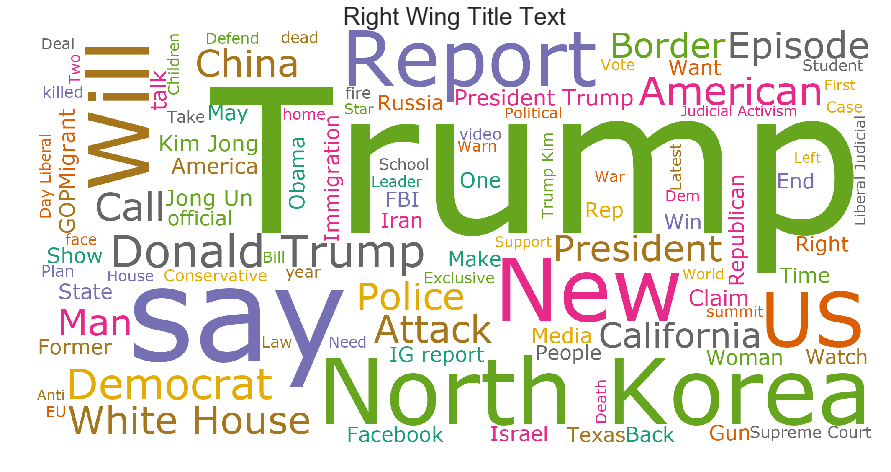
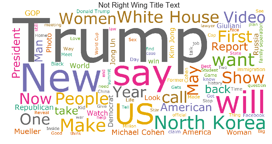
Wordclouds
These provide a nice, fun visualization of words found in right wing and not right wing title text. The larger the word the more it appears.
plt.figure(figsize=(15,8))
wordcloud = WordCloud(font_path='/Library/Fonts/Verdana.ttf',
                      max_words=(100),
                      width=2000, height=1000,
                      relative_scaling = 0.5,
                      background_color='white',
                      colormap='Dark2'

).generate(' '.join(text[right].title))
plt.imshow(wordcloud)
plt.title("Right Wing Title Text", fontsize=24)
plt.axis("off")
plt.show()
plt.figure(figsize=(15,8))
wordcloud = WordCloud(font_path='/Library/Fonts/Verdana.ttf',
                      max_words=(100),
                      width=2000, height=1000,
                      relative_scaling = 0.5,
                      background_color='white',
                      colormap='Dark2'

).generate(' '.join(text[notright].title))
plt.imshow(wordcloud)
plt.title("Not Right Wing Title Text", fontsize=24)
plt.axis("off")
plt.show()
In the next post I will go over the modeling process and evaluation (the fun part!) of this project.
To be continued…